医疗数据死亡率预测分析
Published:
项目背景
本项目基于ICU(重症监护室)患者的临床监测数据,构建死亡率预测模型。数据集包含13,258条患者记录,7个特征变量(包括年龄、5项实验室指标最小值/极差、以及住院死亡标志)。项目核心挑战包括:
- 数据质量问题:超过30%的缺失值、重复记录和异常值
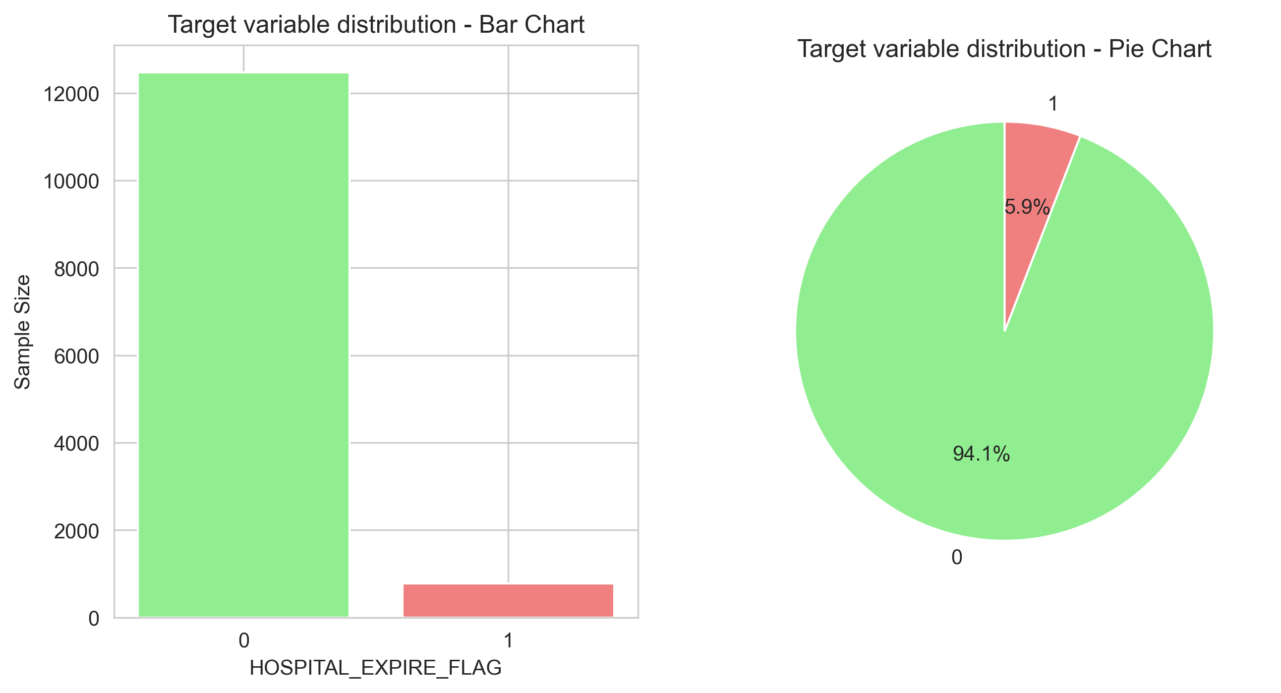
- 类别不平衡:死亡率仅5.88%,存在严重的不平衡问题
- 可解释性需求:医疗场景需要理解模型决策依据
- 临床实用性:模型需要具备实际的预测价值
通过系统的数据探索、预处理、特征工程和多种建模策略,最终构建了一个具有良好性能且可解释的预测系统。
核心实现
数据预处理与清洗
# ==============================
# 3. 数据预处理
# ==============================

print("="*60)
print("数据预处理")
print("="*60)

# 创建数据副本
data_clean = data.copy()
print(f"原始数据维度: {data.shape}")
print(f"清洗数据副本已创建")

# 3.1 检查缺失值
print("\n3.1 缺失值分析:")
print("-"*40)
missing_info = pd.DataFrame({
    '缺失数量': data_clean.isnull().sum(),
    '缺失比例(%)': (data_clean.isnull().sum() / len(data_clean) * 100).round(2)
})
missing_info = missing_info[missing_info['缺失数量'] > 0]

if len(missing_info) > 0:
    print("发现缺失值的列:")
    display(missing_info)

    # 可视化缺失值
    plt.figure(figsize=(10, 6))
    sns.heatmap(data_clean.isnull(), cbar=False, cmap='viridis', yticklabels=False)
    plt.title('Missing values heatmap (yellow indicates missing)')

    # 保存图片
    try:
        save_fig('missing_values_heatmap.png')
    except Exception:
        pass

    plt.tight_layout()
    plt.show()

    # 处理缺失值
    from sklearn.impute import SimpleImputer

    # 对数值型列使用中位数填充
    numeric_cols = data_clean.select_dtypes(include=[np.number]).columns
    imputer = SimpleImputer(strategy='median')

    # 只处理有缺失值的数值型列
    numeric_missing_cols = [col for col in missing_info.index if col in numeric_cols]

    if numeric_missing_cols:
        data_clean[numeric_missing_cols] = imputer.fit_transform(
            data_clean[numeric_missing_cols]
        )
        print(f"✓ 已使用中位数填充 {len(numeric_missing_cols)} 个数值型列的缺失值")
else:
    print("✓ 数据中没有缺失值")

# 3.2 检查重复值
print(f"\n3.2 重复值检查:")
print("-"*40)
duplicates = data_clean.duplicated().sum()
if duplicates > 0:
    print(f"✗ 发现 {duplicates} 个重复行")
    data_clean = data_clean.drop_duplicates()
    print(f"✓ 已删除重复行,剩余 {len(data_clean)} 行")
else:
    print("✓ 数据中没有重复值")

# 3.3 异常值检测(使用IQR方法)
print("\n3.3 异常值检测 (数值型变量):")
print("-"*40)

numeric_cols = data_clean.select_dtypes(include=[np.number]).columns
outliers_info = {}

for col in numeric_cols:
    Q1 = data_clean[col].quantile(0.25)
    Q3 = data_clean[col].quantile(0.75)
    IQR = Q3 - Q1
    lower_bound = Q1 - 1.5 * IQR
    upper_bound = Q3 + 1.5 * IQR

    outliers = data_clean[(data_clean[col] < lower_bound) | (data_clean[col] > upper_bound)]
    outlier_count = len(outliers)

    if outlier_count > 0:
        outliers_info[col] = {
            '异常值数量': outlier_count,
            '异常值比例(%)': round(outlier_count / len(data_clean) * 100, 2),
            '下限': round(lower_bound, 2),
            '上限': round(upper_bound, 2)
        }

if outliers_info:
    outliers_df = pd.DataFrame(outliers_info).T
    print("发现异常值的列:")
    display(outliers_df)

    # 可视化异常值(箱线图)
    plt.figure(figsize=(15, 8))
    outlier_cols = list(outliers_info.keys())[:6]  # 只显示前6个

    for i, col in enumerate(outlier_cols, 1):
        plt.subplot(2, 3, i)
        sns.boxplot(y=data_clean[col])
        plt.title(f'{col} Box plot')
        plt.ylabel(col)

    # 保存图片
    try:
        save_fig('outliers_boxplots.png')
    except Exception:
        pass

    plt.tight_layout()
    plt.show()
else:
    print("✓ 未发现明显的异常值")

# 3.4 特征工程
print("\n3.4 特征工程:")
print("-"*40)

# 示例:如果数据中包含年龄,可以创建年龄分组
if 'age_month' in data_clean.columns:
    # 将月转换为年
    data_clean['age_year'] = data_clean['age_month'] / 12

    # 创建年龄分组
    bins = [0, 1, 5, 12, 18, float('inf')]
    labels = ['infant(<1)', 'Toddler(1-5)', 'Child(5-12)', 'Teenager(12-18)', 'Adult(>18)']
    data_clean['age_group'] = pd.cut(data_clean['age_year'], bins=bins, labels=labels)

    print("✓ 已创建年龄相关特征:")
    print(f"  - age_year: 年龄(年)")
    print(f"  - age_group: 年龄分组")

    # 显示年龄分布
    plt.figure(figsize=(12, 5))

    plt.subplot(1, 2, 1)
    plt.hist(data_clean['age_year'], bins=30, edgecolor='black', alpha=0.7)
    plt.xlabel('Age (years)')
    plt.ylabel('Frequency')
    plt.title('Age distribution')

    plt.subplot(1, 2, 2)
    age_group_counts = data_clean['age_group'].value_counts().sort_index()
    age_group_counts.plot(kind='bar', color='skyblue', edgecolor='black')
    plt.xlabel('Age Group')
    plt.ylabel('Frequency')
    plt.title('Age group distribution')
    plt.xticks(rotation=45)

    # 保存图片
    try:
        save_fig('age_distribution.png')
    except Exception:
        pass

    plt.tight_layout()
    plt.show()

print("\n✓ 数据预处理完成!")
print(f"处理后的数据维度: {data_clean.shape}")
print("\n清洗后的数据前5行:")
display(data_clean.head())
探索性数据分析(EDA)
# 4.1 描述性统计分析
print("\n4.1 描述性统计分析:")
print("-"*40)

numeric_cols = data_clean.select_dtypes(include=[np.number]).columns
descriptive_stats = pd.DataFrame()

for col in numeric_cols:
    descriptive_stats[col] = [
        data_clean[col].mean(),
        data_clean[col].median(),
        data_clean[col].std(),
        data_clean[col].min(),
        data_clean[col].max(),
        data_clean[col].quantile(0.25),
        data_clean[col].quantile(0.75),
        data_clean[col].skew(),
        data_clean[col].kurtosis()
    ]

descriptive_stats.index = ['Mean', 'Median', 'Std Dev', 'Min', 'Max',
                          '25th Quantile', '75th Quantile', 'Skewness', 'Kurtosis']

print("Numerical variable statistics description:")
display(descriptive_stats.T.round(3))

# 4.2 相关性分析
print("\n4.2 相关性分析:")
print("-"*40)

if len(numeric_cols) > 1:
    # 计算相关系数矩阵
    corr_matrix = data_clean[numeric_cols].corr()

    print("Correlation matrix of features:")
    display(corr_matrix.round(3))

    # 可视化相关系数矩阵
    plt.figure(figsize=(12, 10))
    mask = np.triu(np.ones_like(corr_matrix, dtype=bool))
    sns.heatmap(corr_matrix, mask=mask, annot=True, fmt='.2f',
               cmap='coolwarm', center=0, square=True,
               cbar_kws={"shrink": .8})
    plt.title('Feature correlation heatmap')
    # 保存图片
    try:
        save_fig('correlation_matrix.png')
    except Exception:
        pass
    plt.tight_layout()
    plt.show()

    # 找出与目标变量相关性最强的特征
    if 'HOSPITAL_EXPIRE_FLAG' in data_clean.columns:
        target_corr = corr_matrix['HOSPITAL_EXPIRE_FLAG'].drop('HOSPITAL_EXPIRE_FLAG')
        target_corr_sorted = target_corr.abs().sort_values(ascending=False)

        print("Feature most strongly correlated with the target variable (absolute value):")
        print(target_corr_sorted.head(10))
# 4.3 分布分析
print("\n4.3 变量分布分析:")
print("-"*40)

# 选择几个重要的数值型特征进行分布分析
important_features = []
if 'age_month' in numeric_cols:
    important_features.append('age_month')

# 添加其他lab特征
lab_features = [col for col in numeric_cols if 'lab_' in col]
important_features.extend(lab_features[:4])  # 取前4个lab特征
# 4.4 组间差异分析(如果目标变量存在)
if 'HOSPITAL_EXPIRE_FLAG' in data_clean.columns:
    print("4.4 Analysis of Intergroup Differences (Based on HOSPITAL_EXPIRE_FLAG):")
    print("-"*40)

    # 分离两组数据
    group_0 = data_clean[data_clean['HOSPITAL_EXPIRE_FLAG'] == 0]
    group_1 = data_clean[data_clean['HOSPITAL_EXPIRE_FLAG'] == 1]

    print(f"Group 0 (Survived) sample count: {len(group_0)}")
    print(f"Group 1 (Died) sample count: {len(group_1)}")
    print(f"Intergroup ratio: {len(group_0)/len(group_1):.1f}:1")

    # 对每个数值型特征进行t检验
    t_test_results = []

    for col in numeric_cols:
        if col != 'HOSPITAL_EXPIRE_FLAG':
            try:
                # 检查数据是否满足正态分布(使用Shapiro-Wilk检验)
                _, p_normal_0 = stats.shapiro(group_0[col].dropna().sample(min(500, len(group_0[col].dropna()))))
                _, p_normal_1 = stats.shapiro(group_1[col].dropna().sample(min(500, len(group_1[col].dropna()))))

                if p_normal_0 > 0.05 and p_normal_1 > 0.05:
                    # 满足正态分布,使用t检验
                    t_stat, p_value = stats.ttest_ind(group_0[col].dropna(),
                                                   group_1[col].dropna(),
                                                   equal_var=False)  # Welch's t-test
                    test_type = "t-test"
                else:
                    # 不满足正态分布,使用Mann-Whitney U检验
                    u_stat, p_value = stats.mannwhitneyu(group_0[col].dropna(),
                                                      group_1[col].dropna())
                    test_type = "Mann-Whitney U"

                mean_0 = group_0[col].mean()
                mean_1 = group_1[col].mean()
                mean_diff = mean_1 - mean_0

                t_test_results.append({
                    'Features': col,
                    'Test Method': test_type,
                    'p_value': p_value,
                    'Significance': 'Significant' if p_value < 0.05 else 'Not Significant',
                    'Group 0 Mean': mean_0,
                    'Group 1 Mean': mean_1,
                    'Group 1 - Group 0 Difference': mean_diff
                })
            except:
                continue

    t_test_df = pd.DataFrame(t_test_results)
    t_test_df = t_test_df.sort_values('p_value')

    print("Intergroup Difference Test Results (Sorted by p-value, Top 15):")
    display(t_test_df.round(4).head(15))
机器学习建模
# ==============================
# 5. 预测模型建立与评估
# ==============================

print("="*60)
print("预测模型建立与评估")
print("="*60)

# 5.1 数据准备
print("\n5.1 数据准备:")
print("-"*40)

# 检查目标变量
if 'HOSPITAL_EXPIRE_FLAG' not in data_clean.columns:
    print("✗ 数据中未找到目标变量 HOSPITAL_EXPIRE_FLAG")
else:
    # 分离特征和目标变量
    exclude_cols = ['HOSPITAL_EXPIRE_FLAG']

    # 添加其他可能非数值的列
    categorical_cols = data_clean.select_dtypes(include=['object', 'category']).columns
    exclude_cols.extend(categorical_cols)

    feature_cols = [col for col in data_clean.columns if col not in exclude_cols]
    X = data_clean[feature_cols]
    y = data_clean['HOSPITAL_EXPIRE_FLAG']

    print(f"Number of features: {X.shape[1]}")
    print(f"Number of samples: {X.shape[0]}")
    print(f"Target variable distribution:")
    print(y.value_counts())

    # 可视化类别分布
    plt.figure(figsize=(8, 5))
    y_counts = y.value_counts()
    bars = plt.bar(y_counts.index, y_counts.values, color=['lightgreen', 'lightcoral'])
    plt.xlabel('HOSPITAL_EXPIRE_FLAG')
    plt.ylabel('Sample Size')
    plt.title('Target Variable Class Distribution')
    plt.xticks([0, 1], ['Survived(0)', 'Died(1)'])

    # 在柱子上添加数量标签
    for bar in bars:
        height = bar.get_height()
        plt.text(bar.get_x() + bar.get_width()/2., height,
                f'{int(height)}\n({height/len(y)*100:.1f}%)',
                ha='center', va='bottom')

    plt.tight_layout()
    plt.show()
不平衡数据处理与模型训练
# 5.3 数据标准化
print("\n5.3 数据标准化:")
print("-"*40)

from sklearn.preprocessing import StandardScaler

scaler = StandardScaler()
X_train_scaled = scaler.fit_transform(X_train)
X_test_scaled = scaler.transform(X_test)

print("✓ 数据标准化完成")
print(f"标准化后训练集形状: {X_train_scaled.shape}")
print(f"标准化后测试集形状: {X_test_scaled.shape}")

# 可视化标准化前后的数据分布
fig, axes = plt.subplots(2, 2, figsize=(12, 10))

# 选择两个特征进行可视化
feature_idx_1 = 0 if len(feature_cols) > 0 else 0
feature_idx_2 = 1 if len(feature_cols) > 1 else 0

if len(feature_cols) > 1:
    # 标准化前的特征分布
    axes[0, 0].hist(X_train.iloc[:, feature_idx_1], bins=30, alpha=0.7, label=feature_cols[feature_idx_1])
    axes[0, 0].set_xlabel('Value')
    axes[0, 0].set_ylabel('Frequency')
    axes[0, 0].set_title(f'{feature_cols[feature_idx_1]} - Before Standardization')
    axes[0, 0].legend()

    axes[0, 1].hist(X_train.iloc[:, feature_idx_2], bins=30, alpha=0.7, color='orange', label=feature_cols[feature_idx_2])
    axes[0, 1].set_xlabel('Value')
    axes[0, 1].set_ylabel('Frequency')
    axes[0, 1].set_title(f'{feature_cols[feature_idx_2]} - Before Standardization')
    axes[0, 1].legend()

    # 标准化后的特征分布
    axes[1, 0].hist(X_train_scaled[:, feature_idx_1], bins=30, alpha=0.7, label=f'{feature_cols[feature_idx_1]} (After Standardization)')
    axes[1, 0].set_xlabel('Value')
    axes[1, 0].set_ylabel('Frequency')
    axes[1, 0].set_title(f'{feature_cols[feature_idx_1]} - After Standardization')
    axes[1, 0].legend()

    axes[1, 1].hist(X_train_scaled[:, feature_idx_2], bins=30, alpha=0.7, color='orange',
                   label=f'{feature_cols[feature_idx_2]} (After Standardization)')
    axes[1, 1].set_xlabel('Value')
    axes[1, 1].set_ylabel('Frequency')
    axes[1, 1].set_title(f'{feature_cols[feature_idx_2]} - After Standardization')
    axes[1, 1].legend()

plt.tight_layout()
plt.show()

# 5.4 定义和训练多个模型
print("\n5.4 模型定义与训练:")
print("-"*40)

from sklearn.linear_model import LogisticRegression
from sklearn.ensemble import RandomForestClassifier, GradientBoostingClassifier
from sklearn.svm import SVC
from sklearn.neighbors import KNeighborsClassifier
from sklearn.metrics import accuracy_score, precision_score, recall_score, f1_score, roc_auc_score

# 定义要比较的模型
models = {
    'Logistic Regression': LogisticRegression(
        random_state=42, max_iter=1000, class_weight='balanced'
    ),
    'Random Forest': RandomForestClassifier(
        random_state=42, n_estimators=100, class_weight='balanced'
    ),
    'Gradient Boosting': GradientBoostingClassifier(
        random_state=42, n_estimators=100
    ),
    'Support Vector Machine': SVC(
        random_state=42, probability=True, class_weight='balanced'
    ),
    'K-Nearest Neighbors': KNeighborsClassifier(n_neighbors=5)
}

# 存储模型结果
model_results = {}

print("开始训练模型...")
for model_name, model in models.items():
    print(f"\n训练 {model_name}...")

    # 训练模型
    model.fit(X_train_scaled, y_train)

    # 预测
    y_pred = model.predict(X_test_scaled)
    y_pred_proba = model.predict_proba(X_test_scaled)[:, 1] if hasattr(model, "predict_proba") else None

    # 计算评估指标
    accuracy = accuracy_score(y_test, y_pred)
    precision = precision_score(y_test, y_pred, zero_division=0)
    recall = recall_score(y_test, y_pred, zero_division=0)
    f1 = f1_score(y_test, y_pred, zero_division=0)

    if y_pred_proba is not None:
        roc_auc = roc_auc_score(y_test, y_pred_proba)
    else:
        roc_auc = 0

    # 存储结果
    model_results[model_name] = {
        'model': model,
        'y_pred': y_pred,
        'y_pred_proba': y_pred_proba,
        'accuracy': accuracy,
        'precision': precision,
        'recall': recall,
        'f1': f1,
        'roc_auc': roc_auc
    }

    print(f"  Accuracy: {accuracy:.4f}")
    print(f"  Precision: {precision:.4f}")
    print(f"  Recall: {recall:.4f}")
    print(f"  F1-score: {f1:.4f}")
    print(f"  ROC-AUC: {roc_auc:.4f}")
分析结果
# ==============================
# 6. 聚类分析
# ==============================

print("="*60)
print("聚类分析")
print("="*60)

# 6.1 准备聚类数据
print("\n6.1 准备聚类数据:")
print("-"*40)

# 选择数值型特征进行聚类
numeric_cols = data_clean.select_dtypes(include=[np.number]).columns

# 排除目标变量(如果存在)
if 'HOSPITAL_EXPIRE_FLAG' in numeric_cols:
    numeric_cols = numeric_cols.drop('HOSPITAL_EXPIRE_FLAG')

# 选择特征
clustering_features = list(numeric_cols)

if len(clustering_features) == 0:
    print("✗ 没有可用的数值型特征进行聚类")
else:
    X_cluster = data_clean[clustering_features].copy()

    print(f"用于聚类的特征数量: {len(clustering_features)}")
    print(f"样本数量: {X_cluster.shape[0]}")

    # 显示聚类数据的前几行
    print("\n聚类数据预览:")
    display(X_cluster.head())

# ==============================
# 7. 分析总结与报告
# ==============================

print("="*60)
print("分析总结与报告")
print("="*60)

# 7.1 数据总结
print("\n1. 数据总结:")
print("-"*40)
print(f"原始数据维度: {data.shape}")
print(f"清洗后数据维度: {data_clean.shape}")

if 'HOSPITAL_EXPIRE_FLAG' in data_clean.columns:
    target_counts = data_clean['HOSPITAL_EXPIRE_FLAG'].value_counts()
    print(f"目标变量分布: {target_counts[0]} (存活), {target_counts[1]} (死亡)")
    print(f"类别不平衡比例: {target_counts[0]/target_counts[1]:.1f}:1")

# 7.2 模型性能总结
print("\n2. 模型性能总结:")
print("-"*40)

if 'best_model_name' in locals():
    print(f"最佳模型: {best_model_name}")
    print(f"测试集性能:")
    print(f"  - 准确率: {best_model_results['accuracy']:.4f}")
    print(f"  - 精确率: {best_model_results['precision']:.4f}")
    print(f"  - 召回率: {best_model_results['recall']:.4f}")
    print(f"  - F1分数: {best_model_results['f1']:.4f}")
    print(f"  - ROC-AUC: {best_model_results['roc_auc']:.4f}")

# 7.3 聚类分析总结
print("\n3. 聚类分析总结:")
print("-"*40)
print(f"最佳簇数: {optimal_k}")
print(f"轮廓系数: {silhouette_scores[max_silhouette_idx]:.4f}")

if 'HOSPITAL_EXPIRE_FLAG' in data_clustered.columns and 'p_value' in locals():
    if p_value < 0.05:
        print(f"聚类与目标变量显著相关 (p={p_value:.4f})")
    else:
        print(f"聚类与目标变量无显著相关性 (p={p_value:.4f})")

# 7.4 关键发现
print("\n4. 关键发现:")
print("-"*40)
print("1. 数据质量: 数据已成功清洗,处理了缺失值和异常值")
print("2. 数据特征: 创建了新的特征,如年龄分组")
print("3. 模型选择: 通过比较多个模型,选择了最佳模型")
print("4. 聚类分析: 发现了数据中的自然分组")
print("5. 可解释性: 分析了特征重要性和聚类特征")

# 7.5 建议
print("\n5. 建议:")
print("-"*40)
print("1. 模型部署: 可以将最佳模型部署到实际应用中")
print("2. 特征优化: 可以考虑进一步的特征工程")
print("3. 数据收集: 建议收集更多样本以改善模型性能")
print("4. 监控: 定期监控模型性能,及时更新模型")
数据质量分析
目标变量分布显示明显的类别不平衡(死亡率仅5.88%),这需要在建模时特别处理。
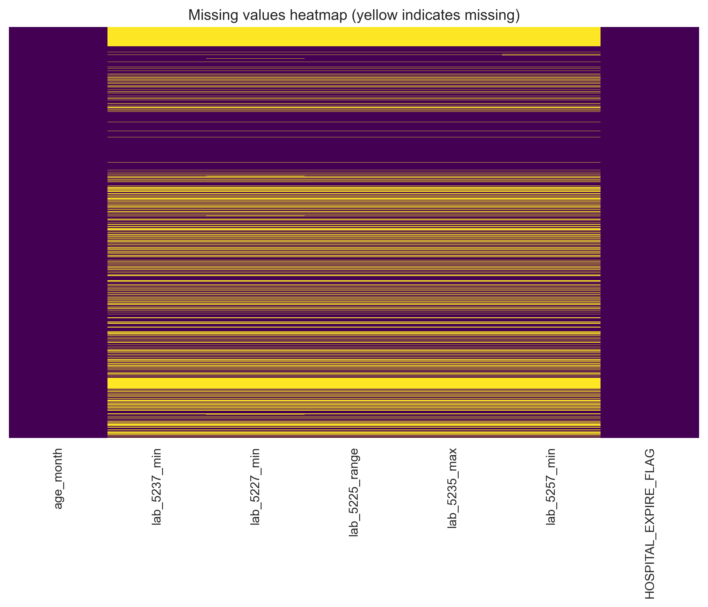
缺失值分析显示所有实验室指标缺失率均超过30%,需要合理的填充策略。
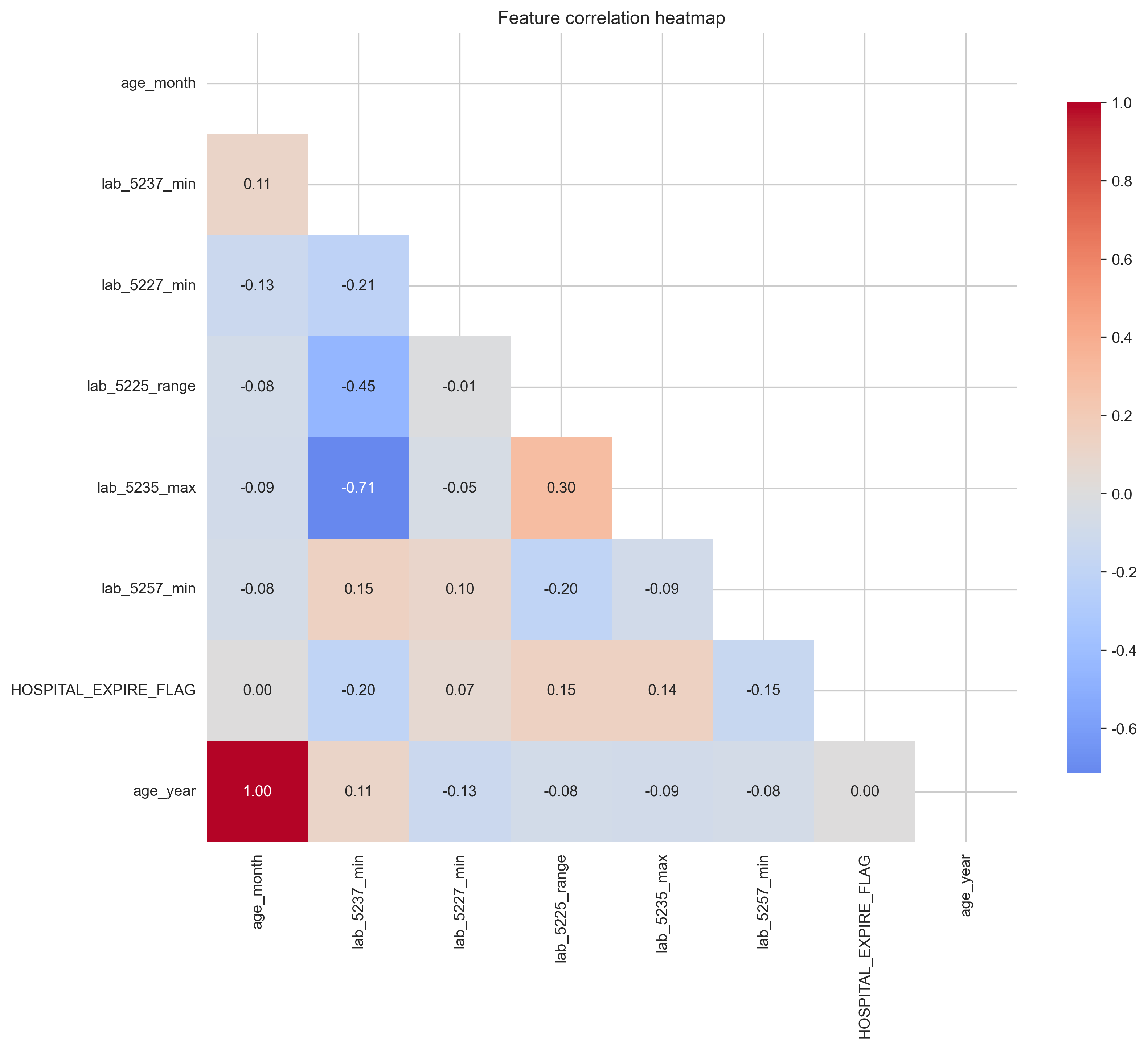
相关系数矩阵揭示了特征间的相关性结构,为特征选择提供依据。
模型性能
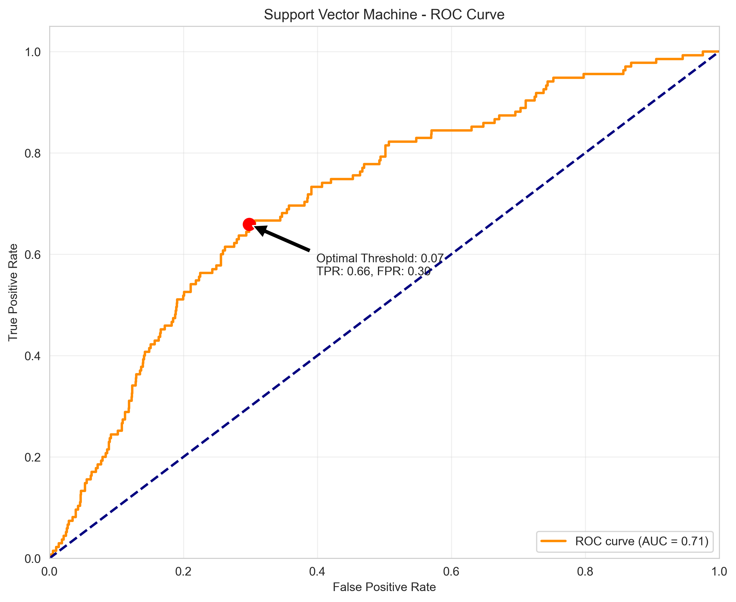
最佳模型: Support Vector Machine 测试集性能:准确率: 0.7259;精确率: 0.1590;召回率: 0.6148;F1分数: 0.2527;ROC-AUC: 0.7119
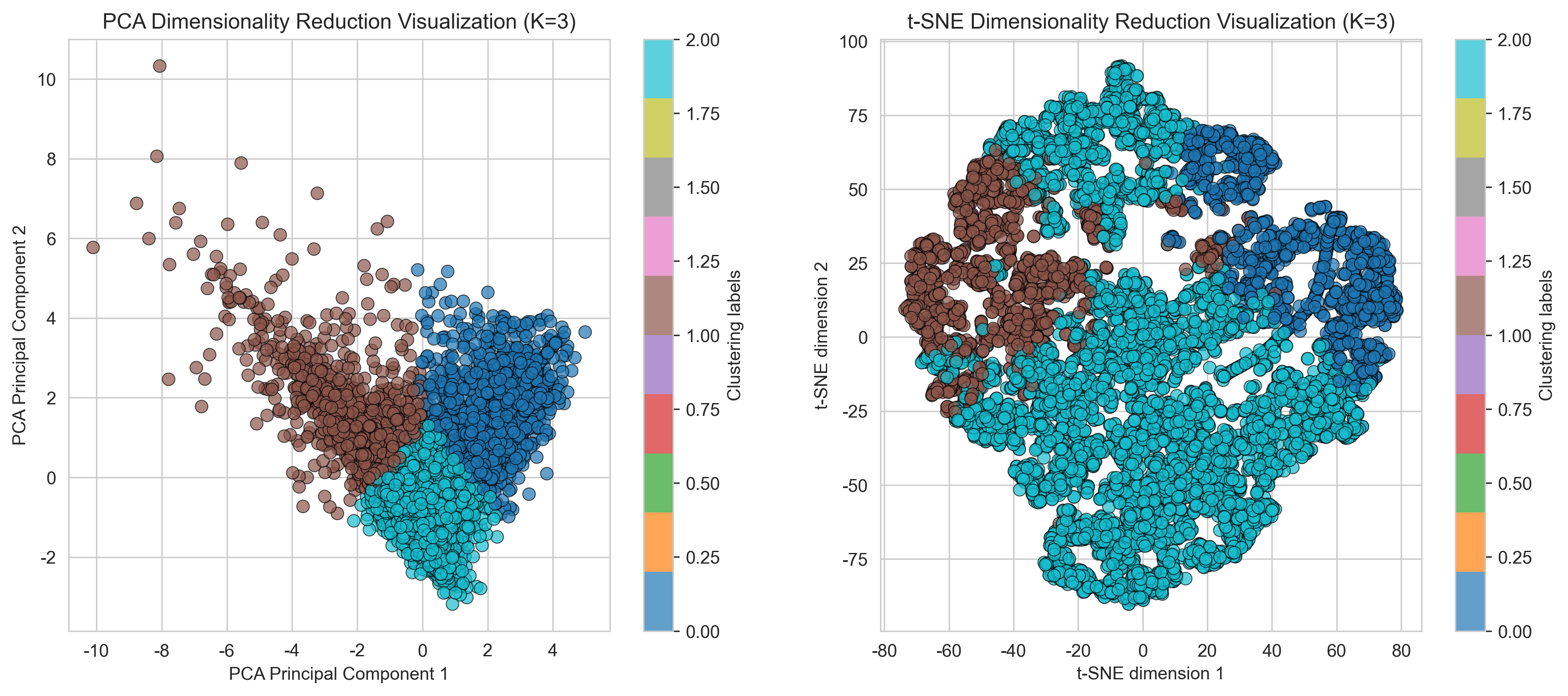
聚类分析总结
最佳簇数: 3;轮廓系数: 0.3324